
Scene Text Detection With Differentiable Binarization
Published:
Introduction
In the real-world, scene text is often with various scales and shapes, including horizontal, multi-oriented and curved text. Segmentation-based scene text detection has attracted a lot of attention in state-of-the-art papers. However, most segmentation-based methods require complex post-processing and take a lot of time in inference phrase. Most existing detection methods use the similar post-processing pipeline as below:
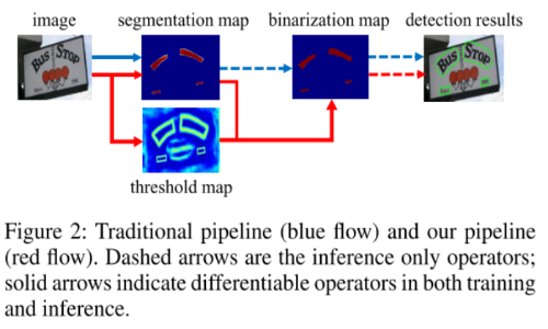
- First, set a fixed threshold for converting the image into a binary image by a segmentation network.
- Then, use some heristic techniques like pixel clustering to group pixels into text instances.
To minimize the set a fixed threshold value, we insert the binarization operation into a segmentation network for joint optimization. The standard binarization function is not differentiable, we instead present an approximate function for binarization called Differentiable Binarization (DB), which is fully differentable when training it along with a asegmentation network.
Binarization
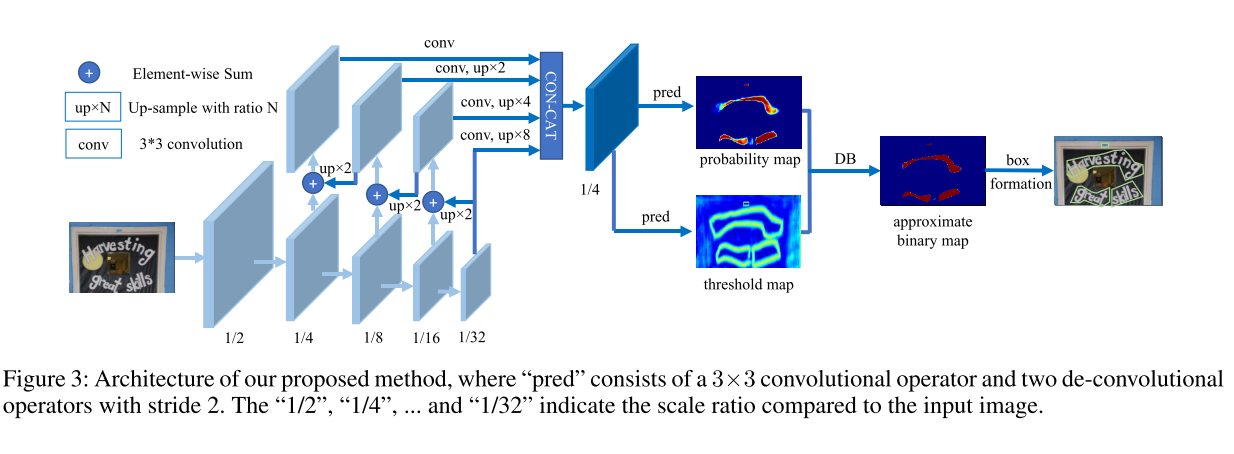
- First, the input image is fed into a feature-pyramid backbone.
- Second, the pyramid features are up-sampled to the same scale and cascaded to produce feature $F$.
- Then, faeture $F$ is used to predict both the probability map $(P)$ and threshold map $(T)$.
- After that, the approximate binary map $(B)$ is calculated by $P$ and $T$.
Standard Binarization
Given a probability map $P \in R^{H\times W}$ produced by a segmentation network, it is converted into a binary map $P \in R^{H\times W}$, with value 1 is considered as valid text areas, otherwise the remaining areas are background with value 0.
\[B_{i, j}= \left\{\begin{array}{rcl}1 & if & P_{i, j} >= t, \\ 0 & otherwise & \end{array}\right.\]where $t$ is the predefined threshold and $(i, j)$ indicates the coordinate point in the map.
Differentiable Binarization
For the standard binarization, it is not differentiable to optimize in segmentation network. To solve this problem, we use a approximate binarization function:
\[\hat{B}_{i,j}=\frac{1}{1+e^{-k(P_{i,j}-T_{i,j})}}\]where $\hat{B}$ is the approximate binarization map. $P, T$ is the probability map and threshold map learned from segmentation network, $k$ indicates the amplifying factor (50 empirically).
Proof the differentiable of $\hat{B}_{i,j}$ in loss function
Set $x = P-T$, $f(x)=\hat{B}$ $\rightarrow f(x)=\frac{1}{1+e^{-kx}}$. We must proof the differentiable of $L_{\hat{B}}=logf(x)$
$\frac{\partial L}{\partial x} = \frac{1}{lne} \frac{1}{1+e^{-kx}} (-ke^{-kx})=-ke^{-kx}f(x)$
So, $L_{\hat{B}}$ is differentiable over all $x \in R$
$\Rightarrow$ what must be proven
Adaptive Threshold
To support for accurate localization of text boders in scences. A technique is designed to apply on threshold map with supervision.

Label generation
I’m impressed with the approach in paper, especially how to create labels for training phase. Many image processing techniques are applied in this paper.
Generation Mechanism

The label generation for the probability map is inspired by PSENet. Given a text image, each polygon of its text regions is described by a set of segments:
\[G=\lbrace S_n \rbrace_{k=1}^n\]$n$ is the number of vertexes (which may be different datasets). Then the positive area is generated by shrinking the polygon $G$ to $G_s$ using offset $D$ of shrinking is computed from perimeter $L$ and area A of the original polygon:
\[D=\frac{A(1-r^2)}{L}\]where $r$ is the shrink ratio, set to 0.4 empirically.
To generate labels for threshold map. Firstly the text polygon $G$ is dilated with the same offset $D$ to $G_d$. The gap between $G_s$ and $G_d$ as the border of the text regions, where the label of threshold map can be generated by computing the distance to the closet segment in $G$ in the training phase.
Experiments on ICDAR2015 dataset
We need to generate labels for probability map and threshold map.
First, the probability map is a binary feature map, the area of texts is value 1, otherwise the remaining areas is background and have value 0. The generation code is implemented in here
Second, the threshold map is gap between the probability map and the dilated probability map (value $\in [0, 1]$). The generation code is implemented in here
Example:
| polygon | probability map | threshold map |
|---|---|---|
 | 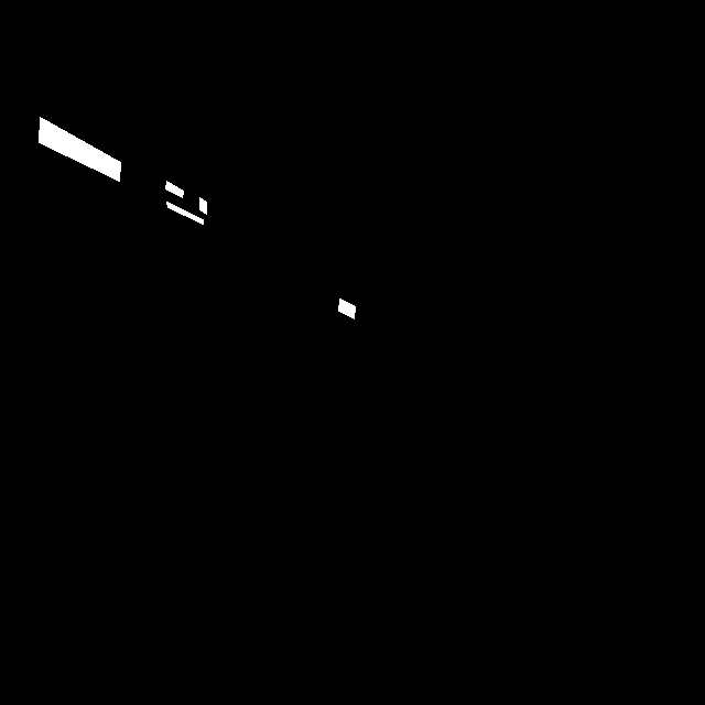 | 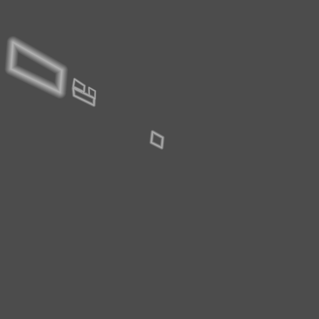 |
Loss function
The loss function $L$ is a weighted sum of the probability map $L_p$, the threshold map $L_t$ and the binary map $L_b$
\[L=L_p + \alpha.L_b + \beta.L_t\]The probability map
The probability map $P \in \lbrace 0, 1 \rbrace$, we apply binary cross entropy loss (BCE)
\[L_p = -\sum^N_i [y_ilog(x_i) + (1-y_i)log(1-x_i)]\]The binary map
The binary map $B \in \lbrace 0, 1 \rbrace$, we also apply binary cross entropy loss (BCE)
\[L_b = -\sum^N_i [y_ilog(x_i) + (1-y_i)log(1-x_i)]\]The threshold map
The threshold map $T \in [0, 1]$, we apply $L_1$ distance loss
\[L_t = \sum_{i \in R_d} = \vert y_i-x_i \vert\]where $R_d$ is a set indexs of pixels inside dilated area that gap between the probability map and the dilated probability map.