SSD: Single Shot MultiBox Detector

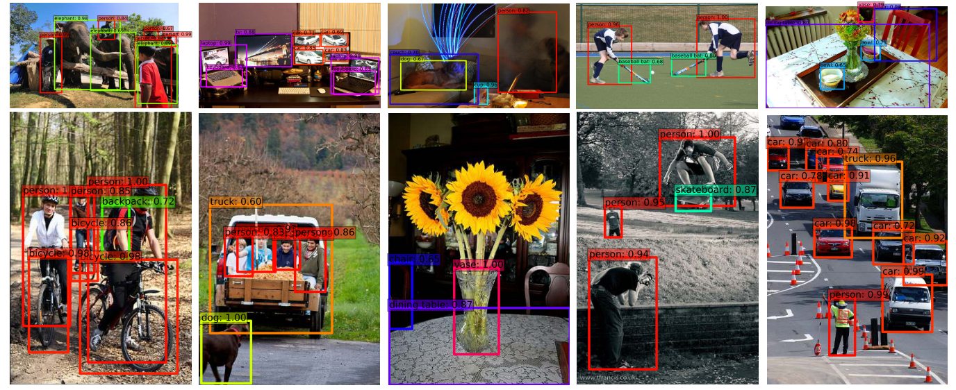
In the object detection algorithm series, I will brifely give a high-level description of everything you need to know about the Pytorch’s implementation of SSD algorithm as described on the SSD: Single Shot MultiBox Detector paper

How does SSD works

SSD uses small convolutional filters applied to feature maps to predict category scores and box offsets for a fixed set of default boxes. To detect objects of different sizes, SSD outputs predictions from feature maps of different scales and explicitly separates predictions by aspect ratio.

During training, we need to first match the groundtruth to the default boxes and then using those matches to estimate the loss function. During inference time, similar prediction boxes are combined to estimate the final predictions.

The Single Shot MultiBox Detector (SSD)

This section decribes the components of SSD architecture

DefaultBoxes Generator

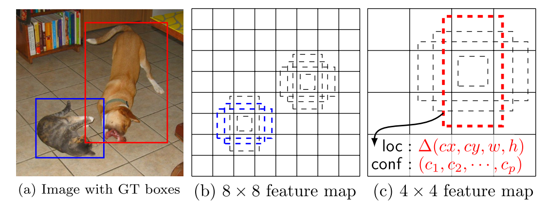
To handle difference object scales, SSD use both the lower and upper feature map for detection. Based on pre-defined feature sizes, the algorithm create a set of default boxes of different espect ratios at each location.

Assume that we want to use $m$ feature maps for detection, the scales of default boxes for each feature map is computed as:

where $s_{min}=0.2$ and $s_{max}=0.9$, and different espect ratios for default boxes denote as $a_r=\lbrace 1, 2, 3, \frac{1}{2}, \frac{1}{3}\rbrace$. The width, height and center for each default box is computed as:

where $\vert{f_k}\vert$ is the size of the k-th square feature map, $i,j \in [0, \vert{f_k}\vert]$. For the aspect ratio of 1, we also add a default box whose scale is $s_k^{\prime} = \sqrt{s_{k} \times s_{k+1}}$ resulting in 6 default boxes per feature map location.

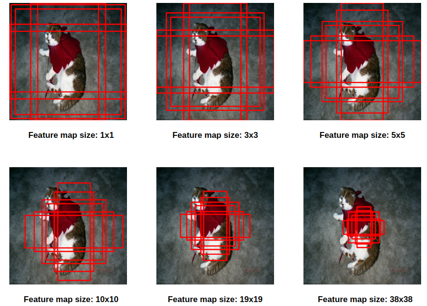
The default boxes are generated at each scale of feature maps aim to predict objects with vary scales (small, medium, large objects). So, we see that at the small feature maps, the model predict large objects and at the large feature maps, the model predict small objects.

Specifically in the example below, the default boxes are generated by DefaultboxesGenerator class :

Matching default boxes

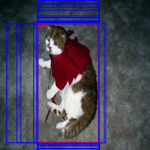
We first match each groundtruth box to the default boxes with the best jaccard overlap higher than a threshold (eg. 0.5). This simplifies the learning problem, allowing the network to predict high scores for multiple overlapping default boxes rather than requiring it to pick only the one with maximum overlap.

Example after applying matching default boxes with threshold=0.4:

Feature Extractor VGG16

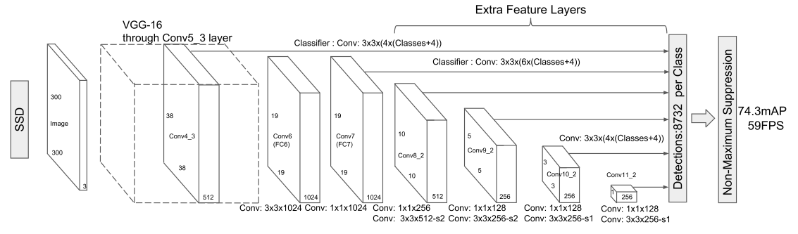
Each added feature layer can produce a fixed set of detection predictions using a set of convolutional filters:

• Feature map 38x38 with conv4_3(FC6): $38 \times 38 \times 4 = 5776$
• Feature map 19x19 with conv7(FC7): $19 \times 19 \times 6 = 2166$
• Feature map 10x10 with conv8_2: $10 \times 10 \times 6 = 600$
• Feature map 5x5 with conv9_2: $5 \times 5 \times 6 = 150$
• Feature map 3x3 with conv10_2: $3 \times 3 \times 4 = 36$
• Feature map 1x1 with conv11_2: $1 \times 1 \times 4 = 4$

Total of default boxes: $5776+2166+600+150+36+4=8732$

Here are a few notable points in Feature Extractor VGG16 implementation:

• Patching the ceil_mode parameter of the 3rd maxpool layer is necessary to get the same feature map size 38x38.
• Change maxpool5 from 2x2-s2 to 3x3-s1 and the use Atrous algorithm.
• L2 normalization is used on the output of conv4_3 to scale the feature norm at each location in the feature map to 20 and learn the scale during back propagation.

Training objective

The overall objective loss function is a weighted sum of the localization loss and the confidence loss:

• The location loss is a Smooth L1 loss between the predicted box and the ground truth box parameters:

• The confidence loss is the softmax loss over multiple classes confidences:

Hard negative mining:

When the number of generated defaul boxes is large, after the matching default boxes step to ground truth boxes, most of the default boxes are negative. We can not use all negative default boxes for optimizing loss, this introduces a significant imbalance between the positive and negative training example. We sort them the highest confidence loss after each computation for each default box and pick the topk with the ratio between the nagative and positive is at most 3:1.

Noteable points in implementation

Representation Encoding with Variance which was never mentioned in the paper

With Lei Mao’s opinion, it is actually a process of standard normalization instead of “Endcoding with variance”. With such many encoded ground truth bounding box representations, we could always calculate the mean and variance of each representation. To achieve better machine learning accuracy, we would like to futher normalize the representation by

Where $\mu_x$ is the mean of variable $X$ and $\sigma_x$ is the standard deviation of variable $X$. In bounding box regression, $\mu_x \approx 0$ in practice. Therefore we could normalize the representations (encoding and decoding the bounding boxes) by

So it should be devided by the standard deviation where $\sigma_x^2 = 0.1$, $\sigma_y^2=0.1$, $\sigma_w^2=0.2$, $\sigma_h^2=0.2$.

Reference

• SSD paper
• Bounding Box Encoding and Decoding in Object Detection