Why is there the concept of cross entropy?

Introduction

Cross-entropy is commonly used in machine learning as a loss function. Cross-entropy is a measure from the field of information theory, building upon entropy and generally calculating the difference between two probability distributions. So how was it built?

What is the Cross Entropy?

Cross Entropy is a measure of the difference between two probability distribution for a random variable or set of events. This concept may sound confusing, I will start with a simple theory to detail understand.

As you know, rare events are more uncertain or more surprising and require more information to represent them than common events. We can calculate the amount of information there is in an event using the probability of the event. This is called self-information or simply the information and can be calculated for a discrete event x as follows:

Where $log()$ is the base-2 logarithm and $p(x)$ is the probability of the event $x$. The choice of the base-2 logarithm means that the units of the information measure is in bits (binary digits). This can be directly interpreted in the information processing sense as the number of bits required to represent the event.

The calculation of information is often written as $h()$; for example:

The negative sign ensures that the result is always positive or zero.

Information will be zero when the probability of an event is 1.0 or a certainty, e.g. there is no surprise.

Consider a flip of a single fair coin.

# calculate the information for a coin flip
from math import log2
# probability of the event
p = 0.5
# calculate information for event
h = -log2(p)
# print the result
print('p(x)=%.3f, information: %.3f bits' % (p, h))
# Output
>> p(x)=0.500, information: 1.000 bits

If the coin was not fair and the probability of a head was instead 10% (0.1), then the event would be more rare and would require more than 3 bits of information.

# probability of the event
p = 0.1
# calculate information for event
h = -log2(p)
# print the result
print('p(x)=%.3f, information: %.3f bits' % (p, h))
# Output
>> p(x)=0.100, information: 3.322 bits

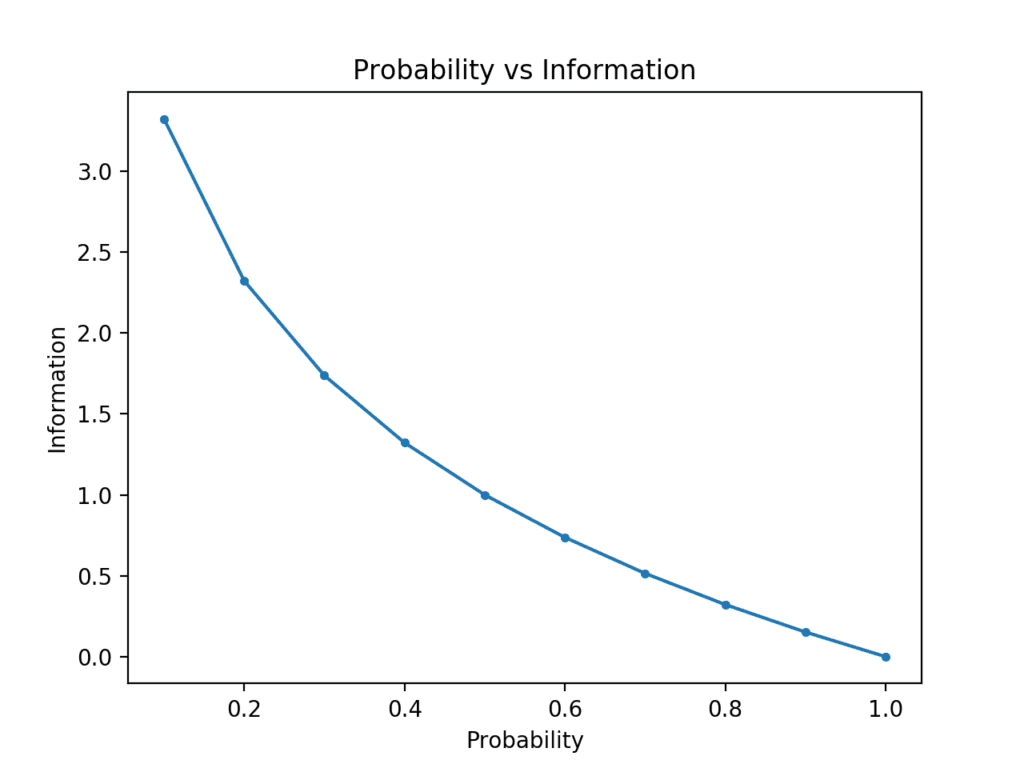
The example creates the plot of probability vs information in bits.

# compare probability vs information entropy
from math import log2
from matplotlib import pyplot
# list of probabilities
probs = [0.1, 0.2, 0.3, 0.4, 0.5, 0.6, 0.7, 0.8, 0.9, 1.0]
# calculate information
info = [-log2(p) for p in probs]
# plot probability vs information
pyplot.plot(probs, info, marker='.')
pyplot.title('Probability vs Information')
pyplot.xlabel('Probability')
pyplot.ylabel('Information')
pyplot.show()

We can see the expected relationship where low probability events are more surprising and carry more information, and the complement of high probability events carry less information.

In effect, calculating the information for a random variable is the same as calculating the information for the probability distribution of the events for the random variable. Calculating the information for a random variable is called Entropy.

Entropy can be calculated for a random variable $X$ with $k$ in $K$ discrete states as follows:

Back to the concept of Cross Entropy, if we consider a target probability $Y$ and an approximation of target distribution $P$, then the cross entropy of $P$ from $Y$ is the number of additional bits to represent an event using $P$ instead $Y$.

The cross-entropy between two probability distributions, such as $P$ from $Y$, can be stated formally as:

Where $Y(x)$ is the probability of the event $x$ in $Y$, $P(x)$ is the probability of event $x$ in $P$ and $log$ is the base-2 logarithm, meaning that the results are in bits.

Cross Entropy as a Loss Function

Cross-entropy is widely used as a loss function when optimizing classification models with:

• Expected Probability (y): The known probability of each class label for an example in the dataset ($Y$).
• Predicted Probability (yhat): The probability of each class label an example predicted by the model ($P$).

We can, therefore, estimate the cross-entropy for a single prediction using the cross-entropy calculation described above; for example.

Where each $x$ in $X$ is a class label that could be assigned to the example, and $Y(x)$ will be 1 for the known label and 0 for all other labels.

The cross-entropy for a single example in a binary classification($c_0$ - class 0, $c_1$ - class 1) task can be stated by unrolling the sum operation as follows:

Example:

# define classification data
p = [1, 1, 1, 1, 1, 0, 0, 0, 0, 0]
q = [0.8, 0.9, 0.9, 0.6, 0.8, 0.1, 0.4, 0.2, 0.1, 0.3]
# calculate cross entropy
def cross_entropy(p, q):
    return -sum([p[i]*log(q[i]) for i in range(len(p))])

# calculate cross entropy for each example
results = list()
for i in range(len(p)):
    # create the distribution for each event {0, 1}
    expected = [1.0 - p[i], p[i]]
    predicted = [1.0 - q[i], q[i]]
    # calculate cross entropy for the two events
    ce = cross_entropy(expected, predicted)
    print('>[y=%.1f, yhat=%.1f] ce: %.3f nats' % (p[i], q[i], ce))
    results.append(ce)
# calculate the average cross entropy
mean_ce = mean(results)
print('Average Cross Entropy: %.3f nats' % mean_ce)

# Output
>>[y=1.0, yhat=0.8] ce: 0.223 nats
>>[y=1.0, yhat=0.9] ce: 0.105 nats
>>[y=1.0, yhat=0.9] ce: 0.105 nats
>>[y=1.0, yhat=0.6] ce: 0.511 nats
>>[y=1.0, yhat=0.8] ce: 0.223 nats
>>[y=0.0, yhat=0.1] ce: 0.105 nats
>>[y=0.0, yhat=0.4] ce: 0.511 nats
>>[y=0.0, yhat=0.2] ce: 0.223 nats
>>[y=0.0, yhat=0.1] ce: 0.105 nats
>>[y=0.0, yhat=0.3] ce: 0.357 nats
>>Average Cross Entropy: 0.247 nats

Reference

• what-is-information-entropy
• cross-entropy-for-machine-learning